Plotting example

library(mixdist)
#> Loading required package: lfstat
#> Loading required package: xts
#> Loading required package: zoo
#> 
#> Attaching package: 'zoo'
#> The following objects are masked from 'package:base':
#> 
#>     as.Date, as.Date.numeric
#> Loading required package: lmom
#> Loading required package: lattice
#> Loading required package: FAdist

Plotting example: Combined plot

This shows how to produce combined frequency plots containing empirical and theoretical distributions (as the one used for Fritz SI in AJS)

Set paths

path1 <- "./inst/extdata/HzbBis2010/" # Austrian data
path <- "./inst/extdata/Bayern_Daten_GL/" # Bavarian Data
plot.path <- "./Plot/" # Plot directory

Load data from Austrian and Bavarian daily discharge monitoring files

The data import uses to read in daily discharges from a typical monitoring file. It returns an ´lfobj´, which is snipped to the reference period: low-flow years starting in April, for the 1950-2010 period.

# Austria (a,c,d)
.pg <-205229 # Ebensee @ Langbathbach - Zone 4 (Flyschzone)
.fi <- paste(path1, "QMittelTag", .pg, ".dat", sep="")
readLines(.fi, n = 5)
x0 <- lfstat::readlfdata(.fi, type="HZB",  hyearstart = 4, baseflow =FALSE)
x2 <- x0[x0$year>=1950,]
x1 <- x2[-(1:90),]
xa <- x1

#b) Bavaria
.pg <- 18381500 # Weg / Isen  ## good!
.path <- "./inst/extdata/Bayern_Daten_GL/"
.fi <- paste(path, .pg, ".dat", sep="")
readLines(.fi, n = 1)
x0 <- readlfdata(.fi, type="LFU",  hyearstart = 4, baseflow =FALSE)
x2 <- x0[x0$year>=1950,]
x1 <- x2[-(1:90),]
xb <- x1

The data objects ´xa´, ´xb´, ´xc´, ´xd´ are available from the package anyway…

Creat plots

width <- 9.5
#x11(width = width, height = width/2)
#or pdf device:
#pdf(file = file.path(plot.path, "Figure_MixedDist.pdf", width = width, height = width/2)

# General plot Layout: 2 horizontal panels
par(mfrow=c(1,2))
par(oma=c(0.5,0.5,2,0.01), mar=c(4,4,0.1,0.1))

Zoomed evplot for Panel a

#b) -> a)
par(mgp=c(2.2,1,0))
# Prepare AM series
AM_list <- seasAM_FUN(xa)
#> Warning: Probably not enough observations to calculate annual minima for the hydrological years:
#> 2010 (58 obs)
AM <- AM_list$AM
# empty plot
evplot(AM, xlab = "-ln(-ln(P(x)))", ylab = "Annual low flow (m³/s)", rp.axis = FALSE, type="n", plim=c(0.001, 0.5), ylim=c(min(AM)-((median(AM)-min(AM))/2),median(AM)))
return.scale.ENG.ZOOM.1()
# draw the plot
ev_plot_combined(AM_list) # Mixed distribution approach
# or: 
ev_plot_combined_COP(xa) # Mixed copula estimator
#> Warning: Probably not enough observations to calculate annual minima for the hydrological years:
#> 2010 (58 obs)
#> Warning: Probably not enough observations to calculate annual minima for the hydrological years:
#> 2010 (58 obs)
mtext("a)", 3, adj=0, line = 0.5)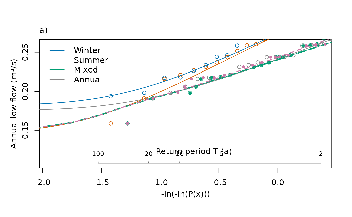

Complete evplot for Panel b

#d)
par(mar=c(4,3,0.1,1.1))
# Prepare AM series
AM_list <- seasAM_FUN(xd)
#> Warning: Probably not enough observations to calculate annual minima for the hydrological years:
#> 2010 (58 obs)
AM <- AM_list$AM
# empty plot
evplot(AM, xlab = "-ln(-ln(P(x)))", ylab = "", rp.axis = FALSE, type="n")
return.scale.ENG.1()
# draw the plot
ev_plot_combined(AM_list)     # Mixed distribution approach
# ev_plot_combined_COP(xd) # Mixed copula estimator
mtext("b)", 3, adj=0, line = 0.5)

And finally close the plot device (especially when plotting a pdf)

dev.off()
#> null device 
#>           1